Von Kármán vortex street Lattice Boltzmann method sim

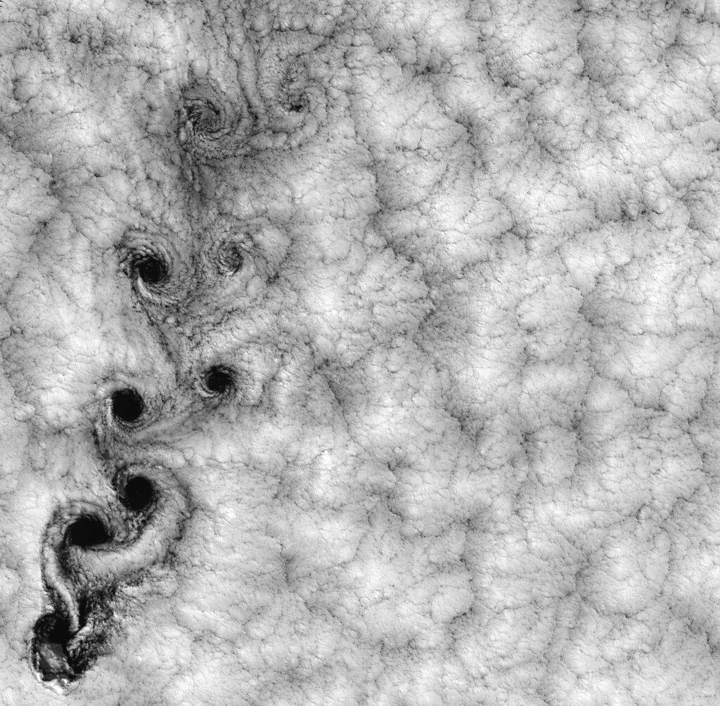
A von Kármán vortex street happens when fluid flows past a cylindrical obstruction. You get a series of vortices that march down flow.

I wrote a Lattice-Boltzmann method solver in c# to simulate such a scenario. It suffers from numerical instability but if the velocity is raised slowly enough, you can reach the top flow speed. For some more information, keep reading below the sim!

I did not write this sim because I was interested in the flow around a cylinder, even though that would be pretty in a high-resolution simulation. I wrote it because I was interested in the Lattice-Boltzmann method, and if you like fluids, you might be too!

There are several fascinating things about this approach. It differs from the kinds of methods I am used to because it doesn’t start from the Navier-Stokes equations. In fact, it simulates the Boltzmann equation. This equation tells us the evolution of a probability distribution \(f(x,t,v)\). This function gives the probability density for a particle with velocity \(v\) at position \(x\) at time \(t\). By taking moments of this distribution you get macroscopic variables, for example the density is given by \(\rho(x,t) = \int f(x,t,v) dv\).

These distributions can change in a gas or liquid for two reasons. The first way is due to the particles moving around or “streaming”. The distribution at \(f(x,t,v)\) will be the distribution at \(f(x+v\Delta t, t+\Delta t, v)\) a small time latter. The second way they can be modified is due to collisions with other molecules. These collisions will mean not all the original particles heading in a direction will get there, some new particles will join and some of the previous particles will change velocity or position. Overall, the actual new distribution will have moved towards some kind of equilibrium state that depends on the macroscopic velocity and density.

This can all be represented wonderfully neatly in the Boltzmann equation:

\[\frac{Df}{Dt} = \Omega(f).\]

Where \(Df/Dt\) is the material derivative (the rate of change following the distribution as it is advected along) and \(\Omega\) is the collision operator. The true collision operator is pretty nasty but the BGK approximation is often used. Under this approximation \(\Omega(f) = -\frac{1}{\tau} (f – f^{eq})\) where \(f^{eq}\) is the equilibrium distribution (a function of the velocity and density at your location) and \(\tau\) is a relaxation rate, or how quickly the distribution tends back to equilibrium due to collisions.

The lattice-Boltzmann equation is the discretisation of the Boltzmann equation onto a lattice. Instead of an infinite range of possible velocities, in a 2D9Q simulation like the one above, the 9 possibilities are the 8 main compass directions and stationary. In 2D9Q, 2D is for 2 dimensions and 9Q denotes the 9 velocities. The Q here is for Yuehong Qian, this is a rare bit of LBM trivia!

This is all well and good, but how do we know that we are really getting the same results as if we discretised the NSE equations directly?

It can be shown that the LBE and NSE match up to order \(O(\Delta t ^2)\). This is done using perturbation theory, there is really not much to fear here. The distribution is Taylor expanded and then moments are taken, this allows for cancellation to occur and it turns out that if you look at the zeroth order terms you have the continuity equation. If you take the first order terms then you can find that setting \(p = \frac{1}{3}\rho c^2\) and \(\nu = \frac{1}{3}(\tau - \frac{1}{2})c^2 \Delta t\) gives the momentum equations. The terms left over are second order so the LBE and NSE are the same up to \(O(\Delta t ^2)\) corrections.

So why does the LBM excite me? I am used to working with spectral methods, these methods are extremely fast for doubly periodic domains but struggle with boundaries. It was fun to use a method that could easily deal with boundaries.

It is also really cool that the LBM is perfect for parallelisation! This makes them an attractive method for anyone with a GPU on their research-grant-funded laptop that they don’t know what to do with.

Finally, the LBM is tantalising because its fundamental unit is not a single value for a velocity, but a probability distribution. Maxwell and Boltzmann managed to capture what was important and discard what was superfluous in thermodynamics. Doing this for a fluid in motion is the great unsolved problem of turbulence. It is interesting to see the two worlds come so close together in a simulation and I wanted a better appreciation for how profound (or not) the approach was. I didn’t have any brain waves while learning about it but hey, maybe you did!

The code I wrote was based on this (much better) Javascript implementation by Dan Schroeder.

By far the best resource I found for understanding the ideas was this course by Amit Gupta!

Until next time