Liouville's equation

Summary

I explain what the Liouville equation for the probability density function (PDF) is and its significance for weather prediction and chaotic systems more generally. I give its derivation, show how it is applied to a simple ODE and the Lorenz 63 system, I discuss its extension to the Fokker-Plank equation and then what relevance Liouville has for weather forecasts.

Introduction

What would the perfect simulation for weather prediction look like? Assuming we are still using the roughly 10 km x 10 km grid boxes of today, it would dutifully track along with the weather we observed in the real world and give a perfect prediction far into the future.

Unfortunately, it is not possible for us to build such a model. There is no way for us to perfectly represent the initial state of the atmosphere in our simulation; we don’t have the resolution and our observations will inevitably have some errors associated with them. That is to say nothing about the model error from our equations being only idealisations of reality and the numerical error inevitably accrued while solving those equations.

The reason our lack of perfectly accurate initial conditions matters is the atmosphere is a chaotic system. Chaotic systems often exhibit a behaviour called sensitive dependence on initial conditions. Arbitrarily small variations in the initial condition can grow to become large differences in the state of the system. This is in contrast to linear systems where the error remains proportional to the initial difference between the true state and its approximation.

In fact, the situation for the atmosphere is even worse than this. At least, with a normal system exhibiting sensitive dependence, the error arbitrarily far into the future can be made arbitrarily small by reducing the initial error. For the atmosphere it is thought that there exists a finite barrier of predictability where no matter how small the initial error is made, after a time period of roughly 2 weeks, the error will saturate and weather prediction skill will drop almost to climatology. Lorenz [1969] labelled this a category III system.

It was eventually appreciated by the weather prediction agencies of Europe and America that any true forecast of the weather must therefore be probabilistic. In 1992 ensemble forecasting methods went into operation at both ECMWF and NCEP. This replaced a deterministic paradigm. Instead of providing a single forecast of the weather, a probability for weather was released.

The ensemble approach is to have, say, 50 realisations of the weather model running with slight differences in the initial conditions. This should give an idea of the spread of weather possible and by counting the number of realisations with a weather feature, the probability of an event. The major difficulty is the huge dimensionality of the problem.

How many numbers do you need to completely represent the state of a weather model? At least 10 million, in newer models perhaps 100 million or more. Each of these numbers is an axis along which the state of the model can be varied, each represents 1 dimension of the configuration space, the state space where the model lives. Suppose we wanted to do a fairly sensible thing and sample our ensemble initial conditions uniformly from an n-dimensional ball around our best guess initial state. To keep things as simple as possible, we represent this by adding 2 states for each of our dimensions. This gives us 2n states to simulate which, for a weather model, is completely impractical.

It is for this reason that a Monte-Carlo ensemble (in this case where 50 members are picked at random from the initial n-ball) will suffer from under dispersion. A small sample is often simply going to miss the more exotic edge cases that lead to the spread we see in the real world. This situation is remedied but not removed through the use of techniques like singular vectors, bred vectors and EDA. These seek to maximise the spread generated by the initial states chosen.

At its heart, an ensemble is an attempt to find the probability density function, \(\rho(X,t)\), of the atmosphere’s state \(X\). The probability density function or PDF is the function that when integrated over a volume in state space, gives the probability the true state lies in that region. For example, \(\int_{\mathbb{R}^n} \rho(X,t) dX = 1\) for all times \(t\).

Could we write down the equation that governs the PDF directly and would solving this provide an alternative to the ensemble approach? The answer to the first question is yes. This is the Liouville equation, the subject of this article. The answer to the second question is probably no as I will discuss in the last section on applications to weather.

Derivation of the Liouville equation

The Liouville equation is the continuity equation for probability. Just as the mass of a parcel of fluid is conserved as it moves along in physical space, the probability associated with a bundle of states is conserved as it moves through configuration space. In a fluid, the continuity equation is \[\frac{D\rho}{Dt} = - (\nabla \cdot u) \rho.\] Here \(\rho\) is the mass density, \(\frac{D}{Dt} = \frac{\partial}{\partial t} + (u\cdot\nabla) \) denotes the material derivative, or the rate of change experienced by a fluid parcel as it is advected by the flow, and \(u = \dot x\) is the velocity.

It should come as no surprise then that the Liouville equation for the PDF \(\rho\) is \[\frac{D\rho}{Dt} = - (\nabla \cdot \dot X) \rho.\]

The most straightforward way to derive this equation is an integral approach. We know that for an arbitrary material volume \(V\) the probability associated with that volume will not change in time:

\[0 = \frac{d}{dt} \int_V \rho dX = \int_V \frac{D\rho}{Dt} + (\nabla \cdot \dot X) \rho dX.\]

Where Reynolds transport theorem was used for the last equality. Since the material volume was arbitrary we know the final integrand must be 0 and so have Liouville.

This glosses over an assumption we are making about the dynamical system we are solving, \(\frac{dX}{dt} = \dot X\). Namely that the Jacobian, which represents the factor by which an infinitesimal volume will be changed as it follows the flow, never becomes negative or infinite. This is equivalent to insisting the evolution map is a one to one map (a bijection).

To spell things out completely then, in the appendix I first show Euler’s identity, that \(\frac{DJ}{Dt} = J \nabla \cdot \dot X\) and use this to prove Reynold’s transport theorem and therefore derive Liouville.

For a Hamiltonian system, \(\nabla \cdot \dot X = 0\) and so the probability density associated with each ensemble member remains fixed. Notice that for a continuous state space, the probability associated with any particular state is always 0, the PDF is a statement about the probability associated with an epsilon ball around a state.

Application to a 1D system

To illustrate the Liouville equation I decided to start with one of the simplest dynamical systems. Consider the autonomous ODE \(\dot x = -x^2 + 5x\). The general term for such a system is a Riccati equation.

The behaviour of the solutions to this system is totally determined by the two fixed points at \(x = 0\) and \(x = 5\). The first is an unstable fixed point and the second a stable one. Solutions that start above 0 will tend asymptotically towards 5 while those that start negative will tend to negative infinity. See figure 1.

Examining this system from an ensemble perspective in figure 2, we see that uniformly sampled initial conditions will bunch up together and then disperse. We can see that this is because the magnitude of \(\dot x\), and therefore the speed that a solution will move, is given by the quadratic \(-x^2 + 5x\). This means that ensemble members will be moving faster if they are on the right initially, spreading out the pack.

If we start with an initial PDF for our system, then we can visualise the evolution of the PDF using Liouville’s equation. We can do this in an Eulerian fashion, where we directly discretise and solve \[\frac{\partial \rho}{\partial t} + \nabla \cdot (\rho \dot X) = 0\] or, as is more practical for systems of higher dimension, proceed in a Lagrangian fashion and solve \[\dot \rho = - (\nabla \cdot \dot X) \rho\] for each ensemble member.

For those unfamiliar with the material derivative, in appendix B I explain how you can see this really does hold in the general n dimensional case using the method of characteristics. In particular, this means we are solving \(\frac{\partial \rho}{\partial t} = -\rho (5 - 2x)\) in figure 3.

Application to the Lorenz 63 system

The Lorenz 63 system is a model of an overturning convective cell stripped back to its essentials. Suppose you fill a hula hoop with air then heat it at the bottom and cool it at the top. The air at the bottom of the hoop becomes less dense as its temperature increases and so rises past the cooler air above it. If the heating is large enough then the air will rise, cool and sink back down on the other side to be heated again with the initial direction the bulk of the fluid circulates being determined by small variations in the initial state.

As the air circulates it will spend more time heating and less cooling. This is because as it heats it will race through the cool upper section and then be slowed down when it reaches the warmer bottom section as it fights against the density gradient. Eventually, it will not cool down sufficiently to sink and will suddenly reverse direction.

The system of differential equations found by Lorenz that approximates this situation was

\[\dot X = -\sigma X + \sigma Y,\]

\[\dot Y = -XZ + rX – Y,\]

\[\dot Z = XY – bZ.\]

With the original values chosen to be \(\sigma = 10\), \(r = 28\) and \(b = 8/3\).

By choosing initial values for X, Y and Z we can solve these equations forward in time and, plotting X in time (see fig 5), we see similar behaviour to that shown in the animation in fig 4.

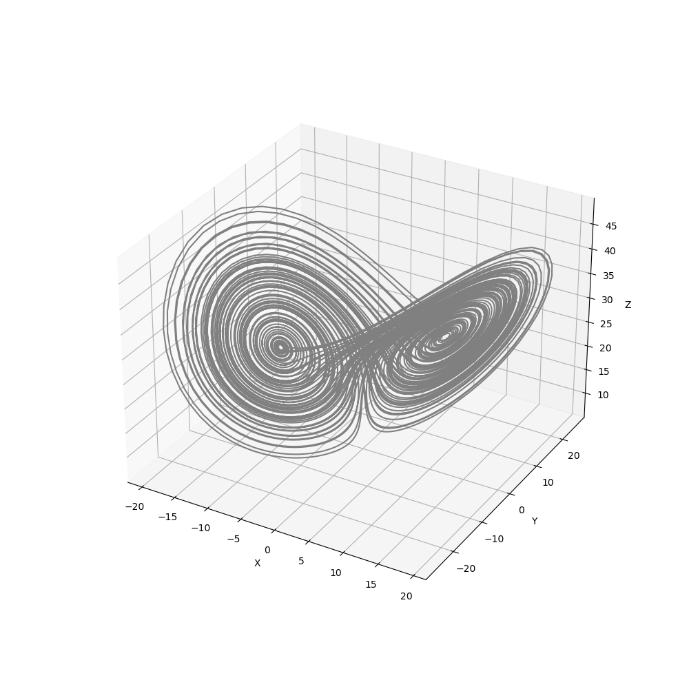
When we visualise not only X but all 3 variables of the problem in time, the butterfly strange attractor is revealed to us as in figure 6 (or at least a trajectory that approaches it). This attractor has become a poster child for chaos theory.

Small differences in the initial state lead to reversals happening at different times. For an ensemble this results in an inevitable spreading out as seen in figure 7.

What happens when we apply Liouville to this system? \(\dot\rho = - \rho \nabla \cdot \dot X\) so calculating the divergence \(\dot\rho = - (-\sigma - 1 - b) \rho\). This means the PDF is exponentially growing.

This is because all the solutions are tending asymptotically towards the 1-dimensional strange attractor. Our 3-dimensional volume in state space is shrinking exponentially along two dimensions even as it is stretched in a third. Another way to look at this is to consider the specific volume \(1/\rho\) which represents the volume occupied by a unit mass (in this case probability). It tends to 0 as time increases and the states get closer to the 0-volume strange attractor.

The animation in figure 8 attempts to show how an initially gaussian estimate for the PDF evolves. The height above the attractor is the value of the PDF.

The Fokker-Plank equation

In deriving the Liouville equation we assumed the evolution map was one-to-one, that is there exists a unique solution for every initial condition. One way this could be violated is if we introduced a random error term. Suppose we wanted to represent the inevitable numerical error we are experiencing. The simplest way to do this would be to introduce a kind of Brownian motion forcing. Our differential equation \(\frac{dX}{dt} = \dot X := F(X)\) then becomes a stochastic differential equation \(dX = F(X)dt + \sigma dW_t\) where \(W_t\) is a Wiener process.

It can be shown through probability theory that the solutions to this SDE have a PDF that obeys the Fokker-Plank equation \[\frac{\partial \rho}{\partial t} = -(\nabla \cdot F(X)) \rho + \frac{\sigma^2}{2}\Delta\rho. \]

This is just the LE equation with a diffusion term.

To evaluate the Fokker-Plank equation requires knowledge of the local terrain of the probability density function (in order to find the Laplacian), this makes its evaluation more difficult than Liouville.

Applications to weather forecasting

Ehrendorfer [1994] noted that “LE provides the basis for making probabilistic statements about specific forecasts”. In practice, the Liouville equation is not used directly in weather prediction.

There are a few reasons for this whose importance depends on the lead time we are interested in. For long lead times solving Liouville is equivalent to finding the strange attractor of the weather. This is presumably a fractal beast living in a very high dimensional space. To find it exactly would be numerically impossible even in the 3-dimensional L63 model. To describe the fully evolved PDF would require an infinite number of statistical moments.

For shorter lead times where the initial PDF has not yet evolved to closely resemble the attractor, the reason it isn't used is fundamentally the high dimensionality of the problem. As mentioned in the introduction, the dimension of state space in a modern weather model is on the order of \(10^8\), making any kind of Eulerian discretisation approach impossible.

Lagrangian approaches (an ensemble might be thought of as a Lagrangian approach) can be used however. Unfortunately, the utility of LE is again hampered by dimension in this case. If we knew the initial PDF of our forecast accurately, then the LE could be used to propagate that information with each ensemble member. This would give us knowledge of the relative confidence we should place in each of the ensemble members. Since the dimension of the system is so large however, the initial PDF is not known with accuracy.

How is the PDF estimated in practice? In the ECMWF ensemble prediction system (EPS) 51 ensemble members are used to estimate the PDF. These ensemble members are not perturbed randomly as in a Monte-Carlo approach. Instead the 25 leading singular vectors are used to ensure that the ensemble members spread out from one another and give a more accurate idea of the range of weather likely. The leading singular vector is the perturbation that can be made to the initial conditions which will cause the maximal error growth to the linearized version of the system in some user defined period of time T.

Conclusion

The Liouville equation is, in a certain way, the fundamental object of study in weather prediction. All our approaches are attempts to approximate the PDF which solves this equation. An ensemble might be thought of as a poor discretisation of the Liouville equation.

Although there are certain advantages to thinking in terms of the Liouville equation, such as the ability to attach some measure of probability to each of the ensemble members, in practical weather applications none of the true challenges have been ameliorated. We still need to integrate our huge system forward in time.

One could imagine LE becoming relevant if machine learning methods or other ideas such as regime dynamics can be used to sufficiently reduce the dimensionality of the weather problem. However, since such approaches will produce evolution maps that are not 1-1, more advanced techniques would be required to find the equations governing the PDF.

Appendices

Appendix A: Derivation of Liouville

The assumption that the evolution map is a one to one mapping is equivalent to assuming the Jacobian \(J\) (which corresponds to local changes in volume in state space following the flow and is a function of time and position in state space) always satisfies \(0 < J < \infty\). That is, a region in state space will never evolve under the flow into nonexistence, or blow up to dominate the whole domain.

Since the evolution is 1-1, we can use Lagrangian coordinates \(X^0\) for any point in state space \(X\). \(X^0\) is the initial state of the position in state space we are looking at at time \(t\).

The Jacobian is then

\[J = \frac{\partial X}{\partial X^0} = \begin{vmatrix} \frac{\partial X_1}{\partial X^0_1} & \frac{\partial X_1}{\partial X^0_2} & ... & \\ \frac{\partial X_2}{\partial X^0_1} & \frac{\partial X_2}{\partial X^0_2} & ... &\... & & & \\ & & & \end{vmatrix}.\]

Now Euler's identity is the result that \(\frac{DJ}{Dt} = J \nabla \cdot \dot X\). This follows since

\[\frac{DJ}{Dt} = \frac{D}{Dt} \begin{vmatrix}\frac{\partial X_1}{\partial X^0_1} & \frac{\partial X_1}{\partial X^0_2} & ... & \\ \frac{\partial X_2}{\partial X^0_1} & \frac{\partial X_2}{\partial X^0_2} & ... & \\ ... & & & \\ & & & \end{vmatrix} \]

\[= \begin{vmatrix} \frac{D}{Dt} \frac{\partial X_1}{\partial X^0_1} & \frac{D}{Dt} \frac{\partial X_1}{\partial X^0_2} & ... & \\ \frac{\partial X_2}{\partial X^0_1} & \frac{\partial X_2}{\partial X^0_2} & ... & \\ ... & & & \\ & & & \end{vmatrix} + \begin{vmatrix} \frac{\partial X_1}{\partial X^0_1} & \frac{\partial X_1}{\partial X^0_2} & ... & \\ \frac{D}{Dt} \frac{\partial X_2}{\partial X^0_1} & \frac{D}{Dt}\frac{\partial X_2}{\partial X^0_2} & ... & \\ ... & & & \\ & & & \end{vmatrix} + ... \\ \]

\[= \begin{vmatrix}\frac{\partial \dot X_1}{\partial X^0_1} & \frac{\partial \dot X_1}{\partial X^0_2} & ... & \\ \frac{\partial X_2}{\partial X^0_1} & \frac{\partial X_2}{\partial X^0_2} & ... & \\ ... & & & \\ & & & \end{vmatrix} + \begin{vmatrix} \frac{\partial X_1}{\partial X^0_1} & \frac{\partial X_1}{\partial X^0_2} & ... & \\ \frac{\partial \dot X_2}{\partial X^0_1} & \frac{\partial \dot X_2}{\partial X^0_2} & ... & \\ ... & & & \\ & & & \end{vmatrix} + ... \]

Where we used that the material derivative keeps \(X^0\) fixed so commutes with derivatives wrt \(X^0\). By applying the chain rule we can see that (since the determinant of a matrix with two copies of the same row is 0) the determinants in the sum are given by

\[\begin{vmatrix}\frac{\partial \dot X_1}{\partial X^0_1} & \frac{\partial \dot X_1}{\partial X^0_2} & ... & \\ \frac{\partial X_2}{\partial X^0_1} & \frac{\partial X_2}{\partial X^0_2} & ... & \\ ... & & & \\ & & & \end{vmatrix}= \frac{\partial \dot X_1}{\partial X_1} \begin{vmatrix}\frac{\partial X_1}{\partial X^0_1} & \frac{\partial X_1}{\partial X^0_2} & ... & \\ \frac{\partial X_2}{\partial X^0_1} & \frac{\partial X_2}{\partial X^0_2} & ... & \\ ... & & & \\ & & & \end{vmatrix} + \frac{\partial \dot X_1}{\partial X_2} \begin{vmatrix} \frac{\partial X_2}{\partial X^0_1} & \frac{\partial X_2}{\partial X^0_2} & ... & \\ \frac{\partial X_2}{\partial X^0_1} & \frac{\partial X_2}{\partial X^0_2} & ... & \\ ... & & & \\ & & & \end{vmatrix} + ...\]

\[= \frac{\partial \dot X_1}{\partial X_1} J.\]

Together this implies indeed that \(\frac{DJ}{Dt} = J \nabla \cdot \dot X\). This result will allow us to prove the equivalent of Reynold's transport theorem.

The probability of us being in a particular ensemble member is fixed. If the evolution map is a bijection then this probability will never alter as time progresses. There will be no other states that feed into ours, increasing the probability of our state.

This means that for any material volume in state space \(V\), the total probability of being within that volume is conserved. We can manipulate this to arrive at LE as follows

\[0 = \frac{\partial}{\partial t} \int_{V} \rho dX\]

\[= \frac{\partial}{\partial t} \int_{V^0} \rho J d X^0\]

\[= \int_{V} \frac{\partial \rho}{\partial t} + (\dot X \cdot \nabla) \rho + \rho \nabla \cdot \dot X d X \]

\[= \int_{V} \frac{\partial \rho}{\partial t} + \nabla \cdot (\rho\dot X) d X\]

Since the material volume is arbitrary we get that \(\frac{\partial \rho}{\partial t} + \nabla \cdot (\rho\dot X) = 0\) and so rearranging have \[\frac{D\rho}{Dt} = - (\nabla \cdot \dot X) \rho. \quad\square\]

Appendix B: Application of the method of characteristics to Liouville

To remind ourselves LE is \(\frac{\partial \rho}{\partial t} + \nabla \cdot (\rho \dot X) = 0\). So \(\frac{\partial \rho}{\partial t} + \nabla \rho \cdot \dot X + \rho \nabla \cdot (\dot X) = 0\). The method of characteristics is to see this equation geometrically. Picture \(X\) as being only a single variables so that the PDF \(\rho(x,t)\) is a surface above the \((x,t)\) plane. The normal to this surface is \((\rho_t, \rho_x, -1)\). We can rewrite our equation as \((\rho_t, \rho_x, -1)\cdot(1,\dot X, -\rho \nabla \cdot (\dot X)) = 0\). I.e., we have a vector that will always lie on the solution surface for \(\rho\). If we use this to step an initial probability distribution forward, parametrising the solution curve with \(\eta\), we have \(t'(\eta)/1 = x'(\eta)/\dot X = -\rho'(\eta)/\rho \nabla \cdot (\dot X)\). Forming differential equations from this we find in general that, given some trajectory in phase space,

\[\frac{\partial x_i}{\partial t} = \dot X \]

\[\frac{\partial \rho}{\partial t} = -\rho \nabla \cdot \dot X.\]

We already knew the first equation. That is just the governing equation for one of our ensemble members. It is our simulation. The second equation is the way the probability density is changing local to our simulation.

References

Ehrendorfer, M. (1994). The Liouville equation and its potential usefulness for the prediction of forecast skill. Part I: Theory. Monthly Weather Review, 122(4), 703-713.

Lorenz, E. N. (1969). The predictability of a flow which possesses many scales of motion. Tellus, 21(3), 289-307.

Lorenz, E. N. (1963). Deterministic nonperiodic flow. Journal of atmospheric sciences, 20(2), 130-141.

Palmer, T. N. (2000). Predicting uncertainty in forecasts of weather and climate. Reports on progress in Physics, 63(2), 71.