Kepler's laws

In this blog, I wanted to trace the history of how we came to know three neat facts about the motion of the planets. These three facts are known as Kepler’s laws, and they are rather beautiful observations that led to the development of classical physics. We will wander through the entertaining history of their revelation and how one can arrive at them from the classical theory of gravity, learning some useful concepts in physics and mathematics as we go. Let us start with what a planet is, or rather, what it was.

Moving the heavens and the Earth: A brief history of Kepler's laws

Planet comes from the Greek word wanderer. Initially, it referred to five mysterious “stars” that seemed to move independently of the fixed starfield of constellations behind them. The names of these five were Mercury, Venus, Mars, Jupiter and Saturn. From our perspective on Earth, the Sun and Moon, as well as the constellations, seem to revolve around us. The planets, however, were harder to explain. They would seem to be moving around us, only to suddenly twist back on themselves in a retrograde motion until they looped back around and continued on their way. 

An early attempt to explain this phenomenon is attributed to Ptomely. Ptomely was a scholar working in the legendary library of Alexandria in 2nd-century Roman-controlled Egypt. He seemed to be a compiler of knowledge, with his grand treatise on the heavens, known today as Almagest, becoming the definitive text on the subject until the 16th century. He explained the motion of the planets as them circling a fixed point that itself was circling the Earth (see Figure 1 for an illustration). However, as more accurate measurements were made, more and more of these circles had to be added in order to match the observations. By the 16th century, the theory had become thoroughly unwieldy. 

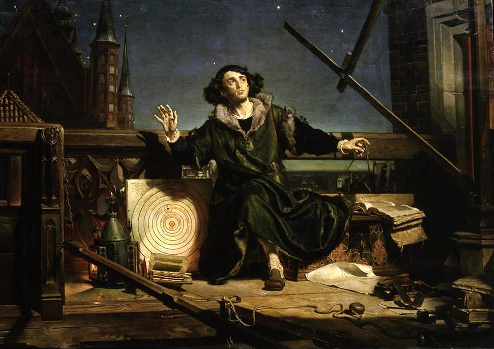
If there is anything for the reader to take away from this article, I hope it is the value of laziness. Had our forebearers continued adding more circles to their theory, they could have explained the observations to arbitrary precision. Even if the orbit of Mars had looked like a vignette of detective Sherlock Holmes from the Earth perspective, the method of epicycles could have been made to match observations with sufficient effort. Thankfully, one man had a conviction that there should be an easier way. 

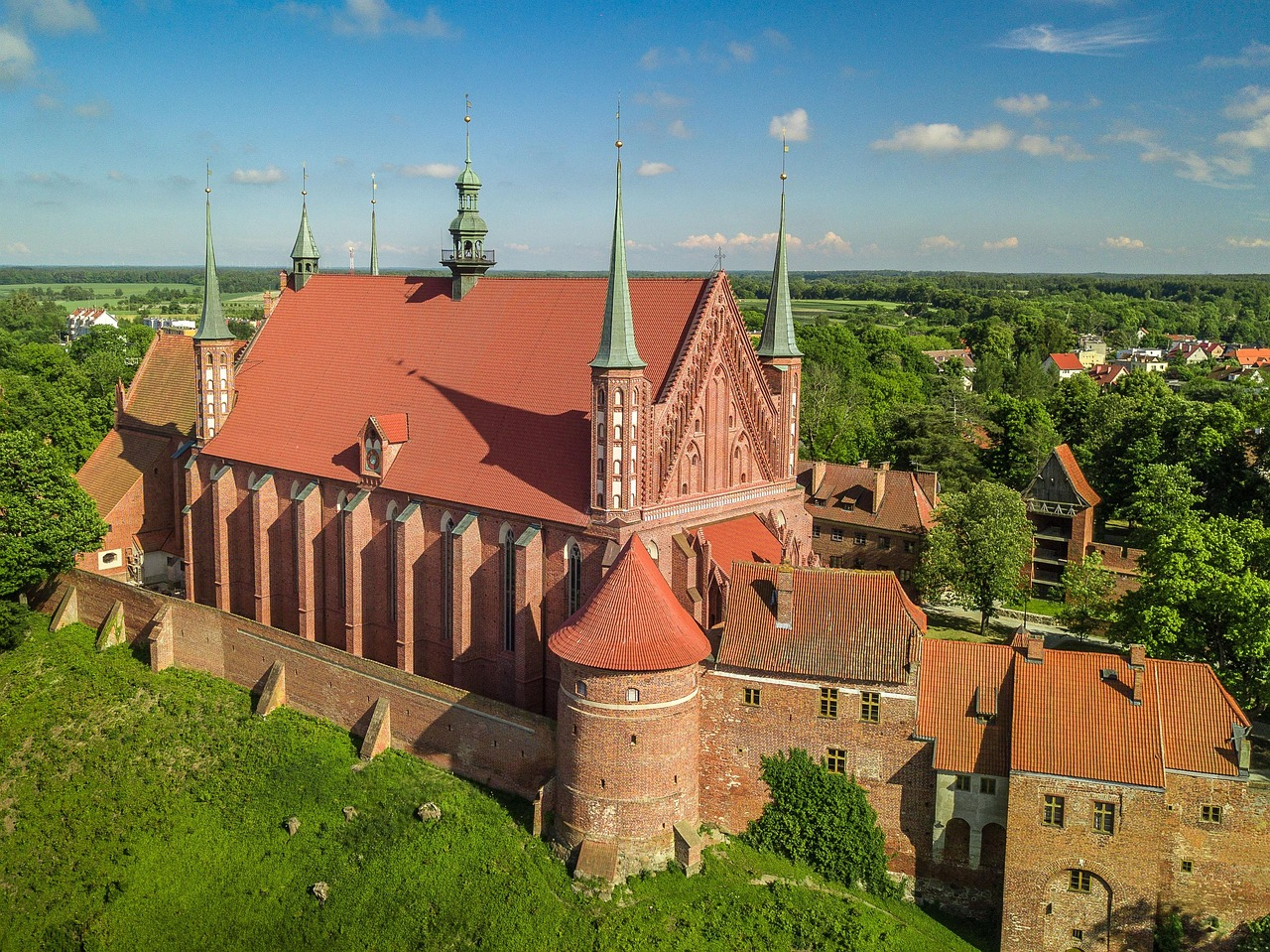
Nicolas Copernicus was born in the Kingdom of Poland. He was educated in Krakow and spent most of his adult life working for the Catholic church in the cathedral of Frombork (Figure 2) - a Polish town very close to the modern Russian enclave of Kaliningrad. In those days, this was quite a significant regional power centre, with Copernicus even being involved in logistics and diplomacy when the Teutonic Order rebelled from 1519 to 1521. 

Copernicus was a multitalented individual. Apart from his main work as a high-ranking official in the church - a church canon - he was also an avid astronomer. With careful thought, he arrived at a simpler explanation for the motion of the planets. He posited that they moved in circles around the Sun, with the Earth moving likewise. When they appeared to move backwards through the sky, all that was happening was the Earth overtaking them in their orbit. We can see this visually in Figure 3.

This elegant explanation was published in De revolutionibus in 1543, which was also the year of Copernicus's death at age 70. I had always assumed Copernicus had purposely timed the publication with his parting, but that doesn’t seem to be the case. Instead, it seems he was gripped with perfectionism rather than fear of reprisal from the church. Indeed, it would be 73 years before the Church would censor Copernicus’s book. This outcome was no doubt helped by the dedication of the book to the Pope and a foreword by its publisher stating it was a mathematical technique rather than a description of physical reality. Although the theory was beautiful, it still did not perfectly explain the observations. To watch the theory fully blossom, it is time for us to venture forward a generation and across northern Europe to Denmark. 

Three years after the death of Copernicus, a Danish nobleman named Tycho Brahe was born. Tycho was an eccentric man; he wore a gold and silver prosthetic nose due to losing his in a duel as a young adult in Germany (it is thought that the duel, which was with another Danish noble, was over a scientific dispute, but the details have been lost to time). Tycho was a devoted astronomer, and made the most accurate naked-eye observations of the sky in history. After falling out with the King of Denmark, Tycho moved his observatory to Bohemia (modern Czech Republic). It was here that he invited a talented mathematician to become his apprentice, Johannes Kepler. 

Tycho, presumably worried about losing recognition for his observational work if they were better analysed by his assistant, was extremely coy with Kepler, only revealing small samples of his observations. This state of affairs continued for around a year until Brahe abruptly died of politeness. Yes, the most common story of his death is that he resisted the urge to relieve himself at a party out of politeness, causing a bladder infection and, shortly after, death. So I suppose the second moral of this article is to be rude as well as lazy. 

Kepler now had access to the observational data he needed. To his consternation, their accuracy thwarted his perfect circular models for celestial motion. After a great deal of trial and error, he succeeded after he dropped the assumption that the motion must be perfect and circular. The planets do not travel in epicycles around the Earth, nor circles around the Sun, but ellipses with the Sun at one focus. This was Kepler’s first law, planets travel in Ellipses. 

Kepler would make two other famous observations about the motion of the planets from Brahe’s data. He would note that the planets sweep out equal areas in equal times (we shall see what we mean by this later) and that there was a harmony in the time it took for a planet to circle the sun and its distance from the sun. 

We are now going to step outside the flow of time and see how these laws emerge from classical physics, which was developed by Newton over fifty years later. Along the way, we are going to discover some useful concepts from Physics and Mathematics. For the mathematically squeamish, have no fear. There is no reason for you not to fear what’s coming, some of it is actually relatively hard maths, I just think you shouldn’t be afraid so much of the time.  

Finding the harmonies in nature: deriving Kepler's laws from classical physics

We are now going to derive Kepler's laws starting from classical physics. The goal of this section is for the reader to come away thinking, "ah, so that's how you derive that". Unfortunately, to meet this goal, a different level of detail would be required for different readers. I will assume that the reader is relatively comfortable with calculus and polar coordinates, is somewhat familiar with the physics of rotation in two dimensions and can take a few things on faith (otherwise, this would quickly become a physics course).

We are going to start with Kepler's first law. This is the hardest one; the other two will be quite quick to cover in comparison.

Conic sections

Conic sections are shapes that can be made by intersecting a plane with a cone (see Figure 4). These are the circle, ellipse, parabola and hyperbola. In order to prove Kepler’s first law, that planets orbit in ellipses, we are going to show that these conic sections are possible solutions to Newton’s law of gravitation applied to two bodies. To do that, we are going to have to be able to recognise a conic section when it introduces itself.

It turns out that we can express these conic sections as points with particular distances from a point and a line (called a directrix). This is shown in the case of a parabola in Figure 5. In particular, we will say that a point is part of our conic section with eccentricity \(e\) if the ratio of the distance to the point and the distance to the directrix is \(e\). That is, assuming the point is the origin, points on our conic section must obey

\[\frac{\textnormal{distance to origin}}{\textnormal{distance to directrix}} = e.\]

Now, the distance between our point and the directrix is just going to be the difference in the \(x\)-coordinate of the line and our point. Let’s let the \(x\)-coordinate of the directrix be \(x\), in polar coordinates, the \(x\)-coordinate of our point will be \(r\cos\theta\). Hence, the distance to the directrix is \(x - r\cos\theta\). So, with a little rearrangement, we have

\[\begin{aligned}\frac{r}{x - r\cos\theta} &= e, \\r + e r \cos \theta &= e x, \\\frac{1}{r} &= \frac{1 + e \cos\theta}{e x}.\end{aligned}\]

This is going to be our smoking gun, if we see the above relationship between \(1/r\) and \(\theta\), we will know we are dealing with conic sections. This is how we are going to prove that planets can orbit in ellipses. 

Radial acceleration 

We will be interested in solving for the trajectory of a body in orbit where the only force it is experiencing is in the radial direction, the attractive force between it and the other body (the Sun), which is at the origin. By Newton’s second law, this means we will be setting \(F=ma\), where \(F\) is the gravitational attraction and \(a\) is the acceleration in the radial direction.

So, we would like to write the radial acceleration in polar coordinates. It won’t all be due to motion in the radial direction, some motion in the orthogonal angular direction will translate into radial motion. Let’s find the formula.

In order to get the radial acceleration, we have to know how our unit vectors in polar coordinates change in time. Our unit \(\mathbf{\hat r}\) vector, will rotate by a tiny step \(\dot\theta\) in the \(\mathbf{\hat \theta}\) direction (orthogonal to \(\mathbf{\hat r}\)). Likewise, \(\mathbf{\hat \theta}\) will also rotate a little in the same way, a direction given by \(-\mathbf{\hat r}\). You can see this illustrated in Figure 6. 

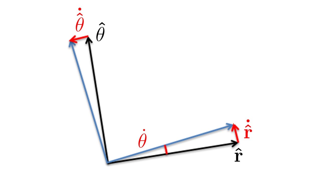
We can gain the insight a little more rigorously by writing \(\mathbf{\hat{r}}\) and \(\mathbf{\hat{\theta}}\) in terms of Cartesian unit vectors \(\mathbf{\hat{i}}\) and \(\mathbf{\hat{j}}\). Then we have 

\[\mathbf{\hat{r}} = \cos\theta \mathbf{\hat{i}} + \sin \theta \mathbf{\hat{j}}\]

and 

\[\mathbf{\hat{\theta}} = -\sin\theta \mathbf{\hat{i}} + \cos \theta \mathbf{\hat{j}}.\]

Differentiating these expressions gives us the result we stated earlier:

\[\begin{aligned}\frac{d\mathbf{\hat{r}}}{dt} &= \dot{\theta} \mathbf{\hat{\theta}}, \\ \frac{d\mathbf{\hat{\theta}}}{dt} &= -\dot{\theta} \mathbf{\hat{r}}.\end{aligned}\]

We can use this to find the radial acceleration term that will be caused by gravitational attraction. So, we can find the acceleration,

\[ \frac{d}{dt} (r\mathbf{\hat{r}}) = \dot{r} \mathbf{\hat{r}} + r \mathbf{\dot{\hat{r}}} = \dot{r} \mathbf{\hat{r}} + r \dot{\theta} \mathbf{\hat{\theta}}, \] 

so we have

\[\frac{d}{dt^2} (r\mathbf{\hat{r}}) = \ddot{r} \mathbf{\hat{r}} + r \dot{r} \dot{\theta} \mathbf{\hat{\theta}} + \frac{d}{dt} (r \dot{\theta}) \mathbf{\hat{\theta}} - r \dot{\theta}^2 \mathbf{\hat{r}}.\]

So in the radial direction, acceleration is: 

\[a = \ddot{r} - r \dot{\theta}^2. \]

Conservation of angular momentum

A curious fact about our universe is there are some numbers you can write down, and no matter what you do, if you do your bookkeeping carefully enough after you do it, you will find that the number has not changed. These are conservation laws. Some are intuitive, such as conservation of energy. Others are harder, like the conservation of colour charge. 

One of the more intuitive ones is conservation of momentum. If a large heavy boulder strikes a very light small rock and comes a complete stop, then the small rock will fly away at great speed as all of the momentum has been transferred to it. This idea of billiard balls or boulders is linear momentum. There is also conservation of angular momentum. If one object is spinning around another, it will not stop doing so until a torque acts on it to arrest the motion. This is the reason the planets orbit the Sun without just falling in. If they were to stop orbiting, it would imply that they lost angular momentum. Since there are no strong forces on them that aren’t in the radial direction, this doesn’t happen (although this situation could change if the other planets conspired to pull the planet in nonradial directions). 

All this is to say that the angular momentum,

\[L = mr^2\dot\theta\]

is a constant. This is going to be extremely useful to us. 

A final little ingredient to showing the 1st law: The fundamental theorem of ordinary differential equations

We are now close to having all the tools we need to tackle Kepler’s first law. Well done if you are still with us, the 1st law is the most difficult. 

We will be constructing and solving an equation involving rates of change in time of positions (accelerations) and fixed positions (distances between attracting objects). Equations like these are called ordinary differential equations or ODEs. In order to solve these equations and find the trajectories that satisfy them, we will be using something called the fundamental theorem of ODEs. 

If we have

\[ y'' + p(x)y' + q(x)y = 0, \] 

which is an equation relating the change of some variable \(y\) which is a function of \(x\) (so \(y\) could be the radial position of a planet and \(x\) could be the angular coordinate) then the fundamental theorem of ODEs says that there is a unique solution to this equation for any initial conditions

\[ y(x_0) = y_0 \] and 

 \[ y'(x_0) = y_1. \]

A consequence of this (although not immediately obvious) is that if we could find two orthogonal solutions to the equation (that is, not somehow the same solution scaled, but two solutions that don’t overlap) then we can construct any solution by combining these two. In particular, this means that if we had two solutions \(y = \cos(x)\) and \(y = \sin(x)\), we can write all possible solutions as \(y = A \cos(x) + B\sin(x)\). This is exactly what we will do later when solving an ODE.

There are two degrees of freedom for our second-order ordinary differential equation. In general, if we look at higher-order ODEs, as in equations with an \(n\)th derivative in them, then there are \(n\) degrees of freedom to the solutions, but we will only deal with second-order equations, so what we have will suffice. 

It’s totally ok if your eyes glazed over a little just now, you don’t need to understand the above deeply to appreciate the derivation that we are about to dive into!

Kepler’s first law

Lucy in the sky with conic sections

We are now going to show that conic sections (and so, in particular, the ellipse) are solutions for the motion of two gravitationally attracting bodies. To do this, we will consider the balance of forces on a planet. 

In perfect equilibrium, a planet will only have a centripetal force provided by gravity acting on it. The force will act at a right angle to its motion and totally explain its acceleration. According to Newton’s second law, \(F=ma\), the radial acceleration of this planet must be given by the law of gravitation by

\[ma = -\frac{GMm}{r^2}.\]

Now, we have just shown in the radial acceleration bit that we can write this in polar coordinates as 

\[ m (\ddot{r} - r \dot{\theta}^2) = -\frac{GMm}{r^2}. \]

Our goal is to solve this differential equation. This is going to be tricky if we have a dependence on both \(r\) and \(\theta\), but luckily we can get rid of the \(\dot \theta\) by rewriting it in terms of the angular momentum. We will then rewrite our ODE in terms of \(1/r\). This is a bit of a trick. You can kind of see why we might want to do this from the sort of terms we have but ultimately, it’s just a way to make our lives easier. So, lets start by using the angular momentum to get rid of \(\dot \theta\), our differential equation becomes:

\[ m \ddot{r} - \frac{L^2}{m r^3} = -\frac{GMm}{r^2}. \]

So rearranging we wish to solve

\[ \ddot{r} = \frac{L^2}{m^2 r^3} - \frac{GM}{r^2}. \]

Now, let’s try that trick we mentioned, we will rewrite the above equation in terms of \(u = 1/r\). We have:

\[ \dot{r} = -\frac{\dot{u}}{u^2} \] 

and

\[ \ddot{r} = -\frac{\ddot{u}}{u^2} + 2 \frac{\dot{u}^2}{u^3}. \]

Substituting this in, this gives

\[ 2 \frac{\dot{u}^2}{u^3} - \frac{\ddot{u}}{u^2} = \frac{L^2}{m^2} u^3 - GM u^2. \]

It’s going to be tricky to deal with \(r\) and \(\theta\) separately, so let's convert all our time derivatives to theta derivatives so that when we solve this equation, we get a formula for \(r\) directly in terms of \(\theta\). To do the conversion, we are going to use the angular momentum again. Rewriting the angular momentum \(L\) in terms of \(u\) we have

\[ L = \frac{m}{u^2} \frac{d\theta}{dt}.  \]

So

\[ \frac{d}{dt} u = \left( \frac{d\theta}{dt} \frac{d}{d\theta}\right) u = \left(\frac{L}{m} u^2 \frac{d}{d\theta}\right) u. \]

Hence,

\[ \frac{d^2}{dt^2} u= \left( \frac{L}{m} u^2 \frac{d}{d\theta} \right) \left( \frac{L}{m} u^2 \frac{d}{d\theta} \right) u \]

\[ = \frac{L^2}{m^2} 2u^3 \left( \frac{du}{d\theta} \right)^2 + \frac{L^2}{m^2} u^4 \frac{d^2 u}{d\theta^2}. \]

So putting this all together, our differential equation in terms of \(\theta\) instead of \(t\) is

\[ \textcolor{red}{ -\frac{L^2}{m^2} 2u \left( \frac{du}{d\theta} \right)^2} - \frac{L^2}{m^2} u^2 \frac{d^2 u}{d\theta^2} +\textcolor{red}{  \frac{2}{u^3} u^4 \frac{L^2}{m^2}  \left( \frac{du}{d\theta} \right)^2} = \frac{L^2}{m^2} u^3 - GM u^2, \] 

where the two red terms cancel each other out. This gives us our ODE to solve:

\[ \frac{d^2 u}{d\theta^2} + u = \frac{GMm^2}{L^2}. \] 

Whew, that was quite a journey. It has taken a lot of work to get to the point where we have a differential equation easy enough for us to go ahead and solve it. An ODE of the form 

\[ \frac{d^2 u}{d\theta^2} + u = \alpha \]

is solved by first finding the homogenous solutions, the solutions to 

\[ \frac{d^2 u}{d\theta^2} + u = 0, \]

and then finding a particular solution for the version with \(\alpha\). This works due to the fundamental theorem of ODEs which I mentioned earlier and the linearity of the equation. If we have two solutions to \(\frac{d^2 u}{d\theta^2} + u = \alpha\) then their difference must solve \(\frac{d^2 u}{d\theta^2} + u = 0\). Hence, we can cover all possible solutions to the system by adding a particular solution to the family of solutions to the homogenous equation.

The family of solutions to the homogenous equation has two degrees of freedom, as discussed earlier, and hence we can look for two orthogonal solutions. Lucky for us, we already know two that fit the bill. The functions \(\sin\) and \(\cos\) become themselves but negative after two derivatives, which is exactly what is required to solve the homogenous equation. Hence

\[ \frac{d^2 u}{d\theta^2} + u = 0 \]

is solved by 

\[u(\theta) = A\cos\theta + B\sin\theta.\]

This has been a long process and so lets cut corners where we can. Instead of explicitly finding \(A\) and \(B\), lets just note that with some basic trig identities, we can rewrite this as 

\[u(\theta) = R\cos(\theta-\theta_0)\]

for some \(R\) and \(\theta_0\).

Now, what is our particular solution? Well, the derivative of a constant is 0, so trivially, \(u = \alpha\) is a particular solution of our actual ODE. Hence, we have found our general solution. It is 

\[u(\theta) = \alpha + R\cos(\theta-\theta_0).\]

And what do we have here? Well, when we looked at conic sections we found that they all looked like

\[\frac{1}{r} = \frac{1 + e \cos\theta}{e x}\]

or put another way

\[u = \alpha + R \cos\theta.\]

Hence, we have shown that solutions for the trajectories of two gravitating bodies under Newton’s laws of gravitation are conic sections. Whether the trajectory is an ellipse, a circle, a parabola or a hyperbola depends on the initial position and velocity of the objects. 

That was the big one, now we can show Kepler’s second law.

Kepler’s second law: Planets sweep out equal areas in equal times

The gif in Figure 7 shows what we mean by Kepler’s second law. In equal periods of time, say one month, the area swept out by an imaginary line connecting the Earth to the Sun is always the same, whether the month we picked to do this was January or July. This neat result can be proved by using the conservation of angular momentum and the formula for the area of a tiny segment.

Consider a circle. The area of a circle is \(A = \pi r^2\). This corresponds to sweeping out an angle of \(2\pi\) in radians. Hence, if the angle we sweep out is \(\theta\), the formula for the area (when we are dealing with a circle) that we sweep out must be \(A = \frac{1}{2}\theta r^2\). But when the angle is small enough, everything is like a circle. Hence, for a tiny change in angle \(\partial \theta\), the corresponding tiny change in area is \(\partial A = \frac{1}{2}\partial\theta r^2\). 

Now, this should look familiar (psst, scroll up to the bit about angular momentum). If we look at the change in angle with time we have

\[\frac{dA}{dt} = \frac{1}{2} r^2 \frac{d\theta}{dt} = \frac{L}{2m}.\]

So the rate of change of area in time is constant and proportional to the angular momentum. Lovely.

Kepler’s third law: the time it takes an object to orbit once depends only on its distance from the Sun

Kepler’s final observation was that there was a harmony between the distance a planet was from the Sun and the time it took to complete an orbit. At first, this may seem trivial, but no matter the mass of the planet, the time it takes to go around depends only on its distance from the Sun. 

The first step to showing this is to recognise that the centripetal force acting on the planet and the force of gravity are one and the same (sorry, I did say I would assume you knew some rotational mechanics). That is

\[mr\dot\theta^2 = \frac{GMm}{r^2}.\]

Now we want to relate \(\dot\theta\) to the period of the orbit. We can do this using Kepler’s second law. We showed that the time it took to sweep out a particular area is constant and equal to 

\[\dot A = \frac{L}{2m}.\]

Hence, the period of the orbit is the time taken to sweep out the area of an ellipse. This gets a bit involved and you need to use the solution we found for the trajectory of the orbit when showing Kepler’s first law. We will instead just show the law for the circle. Where we use the radius in what follows, the actual result is for the semi-major axis of the ellipse. 

For a circle we have \(A = \pi r^2\), so the time for a complete orbit is given by \(T = \frac{2\pi r^2m}{L} = \frac{2\pi}{\dot\theta}\), so 

\[r^3T^{-2} = \frac{GM}{4\pi^2}.\]

Hence, the period of an orbit depends only on the distance from the Sun, and in particular

\[T= \sqrt{\frac{4\pi^2}{GM}} r^{3/2}.\]

This generalises exactly to the ellipse, so that if the semi-major axis is \(a\), the formula for the period of the orbit is 

\[T= \sqrt{\frac{4\pi^2}{GM}} a^{3/2}.\]

Wrapping up

We have just seen three lovely results about the motion of the planets in the sky and how we can derive them from classical physics.

They were:

1. Kepler's first law: Planets move in ellipses

We have seen that, in truth, two bodies interacting via a gravitational attraction can have trajectories that are hyperbola, parabola, ellipses or circles. Which of these is the case is determined by the initial velocities and positions of the bodies. But indeed, counter to the ideas of the time of Planets moving in perfect heavenly circles, they were moving in ellipses, which are still quite attractive.

2. Kepler's second law: Planets sweep out equal areas in equal times

This one is quite a neat result; the area swept out in any unit of time between a planet and its sun is constant. This must have felt like seeing the hand of God in creation for Kepler.

3. Kepler's third law: Planet's orbital periods depend only on their distance from the Sun

Also a very harmonic result. Only the distance from a planet to its star (technically the length of the semi-major axis of its orbital ellipse) is relevant in determining its orbital period. The mass of the planet does not factor into it.

I hope you enjoyed that glimpse into the clockwork of the universe.

Until next time